(Revised for Windows EXCEL 2007)
Project 1 - working with nCr : the
number of combination of r objects taken from a set of n objects
Purpose of this Project:
1. Working with nCr, the number of combinations of r objects taken from a
set of n objects.
2. Entering a formula into Excel.
3. Using the function “COMBIN”.
4. Copying the formula to other cells. Copying maintains relative locations of
variables.
5. Constructing a bar graph (or Chart) in Excel.
Use Internet Explorer on a computer that has Excel installed. All lab computers have Excel installed.
Right click here, and save the file to the desktop. Open with Excel.
The color-coding conventions will be followed on all Excel worksheet for this course. Enter labels into rose-colored cell, enter data into yellow cells, and enter formulas into blue cells.
Instructions.
You will work with, and print out, Sheet 1. There are tabs at the bottom of the
screen for the Sheets.
1. Change the entries in row 1 to your names and section number.
2. In column A, notice that the numbers 0 - 100 have been placed in A6 - A106.
These will be the values of r.
In C5 you will see the label “n = 10”. In this column, starting with row 6, you will enter the values of 10C0, 10C1,
. . . , 10C10.
Here’s how:
select cell C6, then type =combin(10,A6) and hit enter.
OR: select cell C6, then type =combin(10, then click on cell A6, then type ) , and hit enter.
The number "1" should appear in the cell.
.
3. Select the cell C6 again. It will be framed in black; in the lower
right-hand corner of the frame is a small square. As you move the cursor to
this square it changes from a fat "plus sign" to a thin one.
|
|
becomes thin |
4. Select cell C7 and look at the formula at the top of the screen. The A6 has
become A7. Select cell C8, and again look at the formula. Each time the formula
uses the cell in column A that is in the same row as the selected cell.
5. Repeat the process in columns E and G. In column E the formula should be =combin(50,A6) . In column G it should be =combin(100,A6). You will have to copy down to
rows 56 and 106 respectively.
6. Now you are going to make 3 graphs (or charts). Select (highlight) cells C6 - C16. Click on the Insert tab, and in the Charts section, click on Columns. Choose 2-D column (clustered column). A chart will appear. Click on the chart to select (highlight) it and Chart Tools will appear in the Tool Bar. Under Chart Tools, choose the Layout tab. Click on Chart Title and choose Centered Overlay Title. Type 10Cr into the textbox that appears. Make another chart for the entries in column E
(E6 - E56) and one for column G (G6 - G106). Give them the titles 50Cr
and 100Cr, respectively.
Click on the white part of each chart (near "series 1") to move the charts towards the top of the page. Adjust the size of the charts so they fit roughly between columns H and
M.
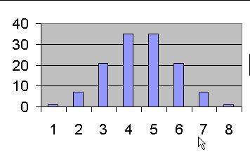
Closing the Gaps
Your graphs (charts) will be spaced out like this:
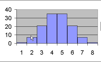
Right click on one of the bars of the chart. Choose Format Data Series. Under Series Options - Gap Width, move the arrow to No Gap.
The
final result should look like this:
Under Series Options - Fill, Border Color, Border Styles, and/or Shadow, make some creative choices. (This is for you to explore the different options.)
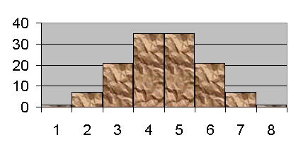
Do this for each of your three graphs.
Printing
On Sheet 1, start with cell A1 and select a region large enough to include all your graphs (but not all the calculated numbers in the columns).
Under the Page Layout tab in the Page Setup section, click Print Area and then Set Print Area.
To the lower right of the Page Setup section, click on the small arrow and a dialog box will appear. Under the Sheet tab, mark "Row and Column headings". You can also check "Print Preview". In order to have print out on one page, you can adjust the margins OR under the Page tab, choose "Fit to 1 page by 1 page" OR under the View tab, choose page break preview and adjust the page breaks.
Print. Bring your printout to recitation on Thursday.