(Revised for Windows EXCEL 2007)

Project 7: Compound Interest Calculator

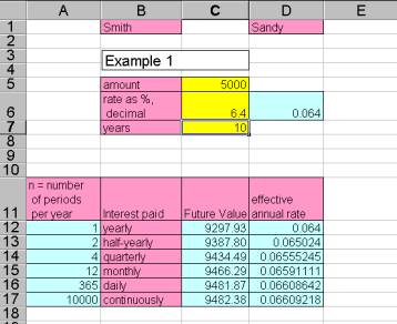
In order to answer questions about compound interest, you will create a spreadsheet that looks like this:

Excel functions and techniques

• Naming a cell – so that all references to the cell will be absolute references
• Formatting a column to always show two decimal places

Math functions:

You will need to enter the appropriate version of this function

Future Value:

where A is the amount deposited, r is the annual rate as a decimal, n is the number of interest periods per year, and y is the number of years.

Effective annual rate:

The effective annual rate, as a decimal, is:

1. Save, then open the spreadsheet (workbook) compoundint2.xls.  Enter your name, etc.
2. In cells D6 , enter a formula which converts the rate in cell C6 to a decimal.
3. In cells A12 – A16, enter the number of interest periods per year. (For continuous compounding, use n = 10,000.)
4. Now you are going to “name” each of the cells: C5, D6, C7. Here’s how to name the cell C5:
   Select C5. Under the Formulas tab and Defined Names, choose Define Name. In the top bar, type Amount. Click on OK.   
   Do the same for the other 2 cells. Here’s a table of the names to use:

C5	Amount
D6	rate
C7	years

5. In cell C12, enter the formula for future value
   =Amount*(1+rate/A12)^(years*A12).
   Instead of pasting this in , type the “equals sign”, then type the rest of the formula, clicking on the cells indicated in bold face.
6. Select cell C12 and drag down the formula.
7. Select cell D12 and enter a formula for the effective rate. Refer to column A for n, the number of periods. Drag down the formula.
8. Finally, let’s fix up the form of the numbers so that there are exactly 2 digits to the right of the decimal point. Select cells C12-C17. Under the Home tab and Cells, choose Format and Format Cells.... Under the Numbers tab, in the Category window on this tab is an entry called “Number”; click that. It should be set to decimal places 2. Click OK (If you want a comma separating the thousands, check that box first).
9. If you set the values in cells C5-C7, to match the example above, your results should also match.
10. Save the workbook.
11. There are three questions on Sheet 2 of the workbook. (The sheet is named “questions”.) Use the interest calculator you have created to answer the questions. Remember to Paste Special – Values (or else the answers will change!).
12. Print the spreadsheets: Sheet 1 (compound interest calculator) and Questions.